> For the complete documentation index, see [llms.txt](https://docs.lenderlink.ph/llms.txt). Markdown versions of documentation pages are available by appending `.md` to page URLs; this page is available as [Markdown](https://docs.lenderlink.ph/backtesting-guides/back-testing-process/lenderlink-data-predictive-power-assessment.md).
# LenderLink Data - Predictive Power Assessment
## LenderLink Data – Predictive Power Assessment
### Introduction
The purpose of this document is to help potential LenderLink clients assess the results from historical back-testing. By understanding the key evaluation metrics and the methodology behind them, clients can make informed decisions about integrating LenderLink data into their credit assessment processes.
### Evaluating Results
#### Hit Rate
**Definition**\
Hit Rate represents the proportion of a client’s borrowers for whom LenderLink was able to retrieve at least one corresponding record from its database.
**Calculation**

**Interpretation example**\
If a client has 10,000 loans and LenderLink data is available for 6,000 of them, the hit rate is 60%. This means that risk signals can be evaluated for 60% of the portfolio.
***
#### Information Value (IV)
**Definition**\
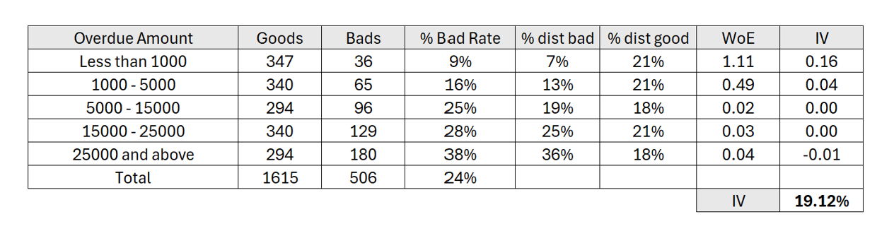
Information Value (IV) measures the strength of the relationship between a single explanatory variable and a binary outcome (e.g. good vs. bad). It assesses how well a variable distinguishes between outcomes based on the distribution of good and bad borrowers across predefined bins.
IV is primarily used for **variable assessment and early-stage screening**, rather than for evaluating overall model performance.
**How IV is calculated**
1. Divide the variable into bins (e.g. deciles or business-defined ranges).
2. For each bin, calculate:
* Share of good borrowers
* Share of bad borrowers
3. Compute Weight of Evidence (WoE).\

4. Aggregate the bin-level contributions to obtain IV.\

**Interpretation guidelines**
| IV Range | Interpretation |
| ----------- | ----------------------- |
| < 0.02 | Not predictive |
| 0.02 – 0.10 | Weak predictive power |
| 0.10 – 0.30 | Medium predictive power |
| > 0.30 | Strong predictive power |
**Example**\
When analyzing a variable such as *Overdue Amount*, higher overdue ranges often contain a disproportionately larger share of bad borrowers. This divergence between good and bad distributions leads to a higher IV, indicating that the variable is informative for credit risk assessment.
**Practical note**\
IV is a univariate measure and does not capture interaction effects, incremental contribution alongside existing model features, or monotonic risk ordering. Variables with a clear monotonic relationship to risk may therefore show relatively low IV despite being predictive.
***
#### Gini Coefficient
**Definition**\
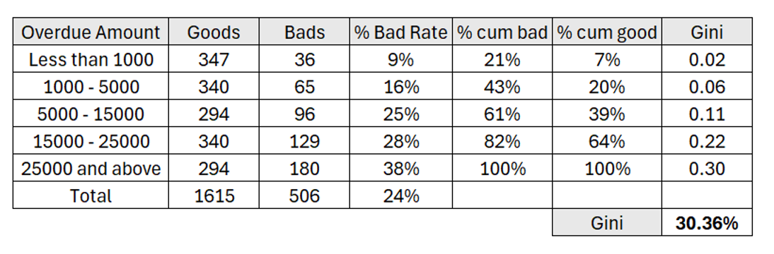
The Gini coefficient measures how well a variable or model separates outcomes across a population. It quantifies discriminatory power by evaluating how consistently risk changes across ordered values.
**Calculation approach**
**Interpretation (Philippines context, single variables)**
| Gini Range | Interpretation |
| ------------- | ----------------------- |
| 0–5% | Low predictive power |
| 5–25% | Medium predictive power |
| 25% and above | High predictive power |
**Example**\
Using the same *Overdue Amount* variable, the Gini coefficient captures how consistently default risk increases as overdue balances rise. Even when Information Value is moderate, a clear monotonic trend can result in a higher Gini, highlighting stronger discriminatory power.
**Gini for scores**\
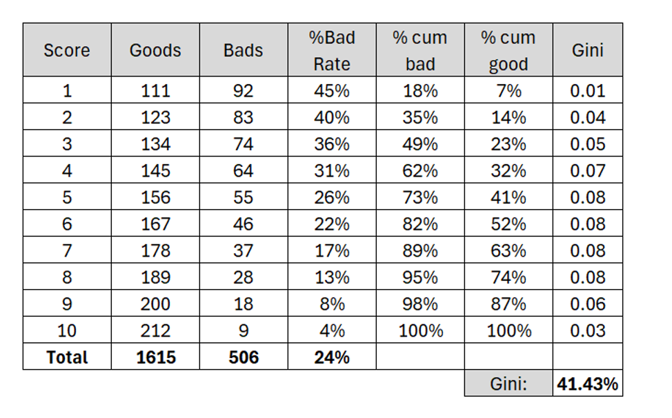
The same concept applies to scoring models. Gini can be calculated on predicted scores to assess the overall discriminatory power of a model, including when combining LenderLink-derived features with an existing internal score.
### Recommended Evaluation Approach
LenderLink data reflects borrower behavior across multiple loans and lenders and should be evaluated for **incremental predictive value**, rather than in isolation.
#### Overlay (Challenger) Model
* Keep the approved production model unchanged
* Build a challenger model combining the existing score with LenderLink features
* Evaluate incremental lift using:
* Change in Gini / KS
* Bad rate at constant approval rate
#### Risk Segmentation
* Select an approved population or a narrow score band
* Use LenderLink data to further segment borrowers
* Assess:
* Bad rate monotonicity
* Risk separation across segments
#### Live Proof of Concept (POC)
* Run LenderLink in parallel with production decisions
* No impact on approvals or declines
* Analyze outcomes after a sufficient observation period
#### Key Metrics to Monitor
* Change in Gini / KS
* Bad rate reduction at constant approval
* Approval uplift at constant bad rate
* Segment-level risk separation